Defending Against a Declining Dollar: Has the US Dollar Bear Emerged From Hibernation?
Key Takeaways
- Bond investors can experience positive returns in an environment with rising interest rates.
- During both the 2001-2007 and 2001-2008 periods, the non-US dollar fixed income benchmarks (in particular, emerging markets and non-US dollar bonds) exhibited attractive risk-adjusted returns and favorable performance.
- International non-US dollar bonds can give investors diversification and return benefits as part of their comprehensive asset allocation. They can also help preserve investors’ purchasing power during a US dollar decline and help to preserve capital in a diversified portfolio.
- US dollar-denominated global bonds offer a compelling diversification component, as measured by their high Sharpe Ratio metrics and favorable returns. However, the asset class does have higher volatility, as measured by standard deviation.
- US dollar-denominated emerging market bonds exhibit as much volatility as US Corporate High Yield bonds, so investors need to manage their expectations and use a longer-term outlook if investing in this asset class.
By the fourth quarter of 2020, investors realized the US dollar had been declining for the past several months. From mid-May's high of 100.47, the US Dollar DXY Index dropped 6.25% to 93.86 by the end of the third quarter. Investors began constructing scenarios to explain the weakness, with extra attention on Georgia’s senate elections, which paved the way to Democratic control of government, opening the door to aggressive stimulus. Despite Federal Reserve chai man Jay Powell’s assurances that any inflation arising from the stimulus combined with pandemic recovery would be short-lived, the potential corrosive effect of inflation on the dollar remains top of mind. Of course, since its nadir on January 5, the US dollar has been recovering, though volatility remains an issue.
How should investors interpret the US dollar’s gyrations? Does the modest price movement during the fourth quarter of 2020 represent the extent of the dollar’s decline, or does it foretell of more to come? The market has a nickname for an investor who believes the dollar will decline: a US dollar bear. Will the US dollar bear emerge from hibernation in the coming spring and summer, or should we expect it to simply continue its slumber?
More importantly, what can investors do to protect themselves if we do face a US dollar decline?
The Previous US Dollar Bear Market, 2001-2008
We can look to history to offer a guide, if not a possible road map of how a US dollar bear market adversely affected investors and consumers.
The previous US dollar decline lasted about seven years, beginning in 2001 and ending in the summer of 2008. During that time, the relative value of the dollar decreased -39%, or -7% compounded annually. Over the same period, inflation, as measured by the Consumer Price Index (CPI), averaged 3% annually, well above the Federal Reserve’s target rate of 2%. Over the same period, the prices of key household items increased; for example, a gallon of milk rose 3.8%, while gasoline rose 14.2%.
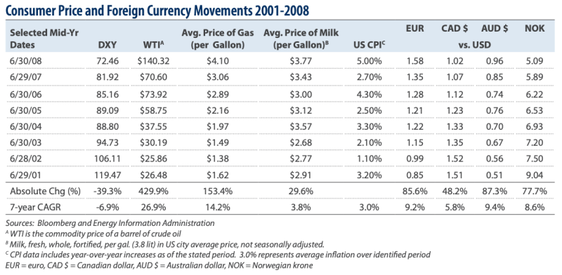
As a result of the inflation, US consumers experienced a meaningful purchasing power decline, which accelerated toward the end of the decade as the CPI rose by an average 3.9% during the latter three years.
Unless an individual’s earnings grew at least the same rate as inflation, their purchasing power declined due to the rising prices. While consumers’ budgets may not have changed in nominal terms, the lower value of the dollar caused budgets to shrink in real terms.
The Great Financial Crisis (GFC) began in the first half of 2008, when financial assets and home prices experienced a pronounced decline and job losses skyrocketed. During the GFC, grocery stores and other retail industries began implementing gas surcharges and fees to offset the accompanying rapid rise in gas prices. This only further diminished the purchasing power of US consumers. The price of crude oil, expressed as Western Texas Intermediate (WTI) in the Consumer Price and Foreign Currency Movements 2001–2008 chart, nearly doubled from June 2007 to June 2008. The entire supply chain of key household items was adversely affected by the precipitous rise in the cost of oil and falling consumer incomes. Real household median income declined by almost -10% from 2007 to 2012, and real median household net wealth fell by -40% from 2007 to 2013.2
Other currencies such as the euro, the Canadian dollar, and the Australian dollar appreciated relative to the US dollar. The euro appreciated at a seven-year CAGR of 9.2%, the Canadian dollar rose at a 5.8% clip, and the Australian dollar by 9.4% annually. In effect, the US dollar bear market reduced US consumers’ ability to afford goods from those regions. While the GFC impaired developed economies around the world, foreign currency appreciation against the US dollar helped offset some of the purchasing power decline for residents of those respective countries. Global commodities are generally priced in dollars so rising gasoline and other prices for an American consumer presented less of a problem for consumers in other countries.
Similarly, investing in a diversified portfolio that includes foreign securities priced in foreign currencies can be an effective way to preserve purchasing power.
Examining the Causes of the Last US Dollar Bear’s Awakening
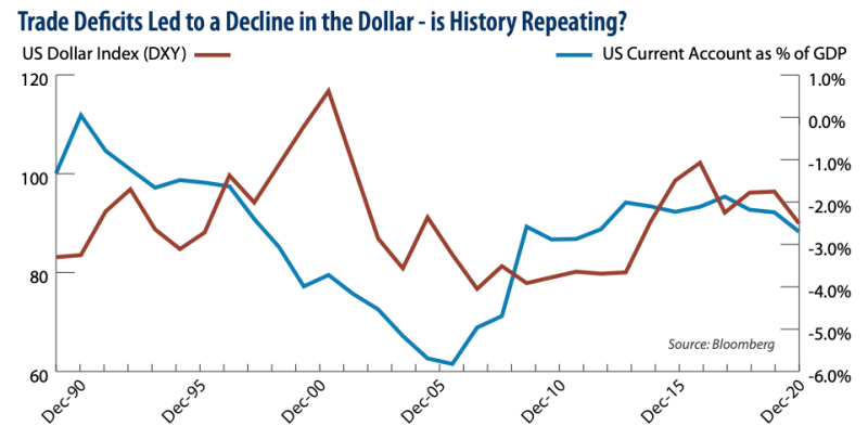
A number of causes and conditions can lead to the decline of a country’s currency, including rampant domestic inflation, weak economic growth, large trade deficits, loose fiscal policies, deteriorating fiscal deficits, and increasing debts. In the United States, currency decline is further complicated by the US dollar being the world’s reserve currency. The dollar and euro combined are the leading mediums of exchange, accounting for about three-quarters of international payments for cross-border trade and financial transactions. As a result, there are numerous complicating factors when a country’s currency is a reserve currency.
The decline of the US dollar from 2001 to 2008 has largely been attributed to an unprecedented US trade deficit, which grew in excess of 5.5% of GDP in 2006.4 Large trade deficits caused an imbalance that led to a circuitous decline in the US dollar and had “the effect of pouring massive amounts of US dollars into the world, which in turn, pushes down the value of the dollar,“ authors Jones and L’Oste-Brown assert in their book, The Devaluation of the United States Dollar: Causes and Consequences.
They continue by arguing that as countries that produce higher priced commodities, such as oil and minerals, began to accumulate vast reserves of US dollars, they began redirecting their allocations to investments that offered a more compelling post-currency adjusted return. “An insufficient inflow of dollars back into the US leads to further depreciation of the dollar.”5 The supply-demand imbalance that resulted from the over-availability of the US dollar was a major factor in the 2001-2008 decline.
Assessing Current Conditions – Is the Hibernation Over?
The central arguments among investors during the fourth quarter of 2020 point to another supply-demand imbalance. This time, they say, the imbalance would result from government spending, budget deficits, and debt rather than from a growing current account balance deficit. In simple terms, the US’s fiscal house is in disarray following the pandemic’s adverse economic impact. The expected outcome is an increase in the supply of US dollars.
Fortunately, we can examine the potential US dollar decline by reviewing other investment playbooks for guidance. Investment and currency trading icon, Stanley Druckenmiller, along with his former boss, George Soros, CEO of Soros Fund Management, earned notoriety when they “broke” the Bank of England on September 17, 1992, referred to now as “Black Wednesday.” The trade reflected an epic event in foreign exchange markets as the Bank of England purchased £27 billion of its own currency in a failed attempt to offset the tremendous selling brought by Soros’ hedge fund, the Quantum Fund. As a byproduct of the “currency attack,” the Quantum Fund earned close to a $1.0 billion profit. The English pound fell -15% against the German mark and -25% against the US dollar.6 In an interview for the book The New Market Wizards, Druckenmiller theorizes that if a country engages in expansionary fiscal policy while engaging in tight monetary policy, one could expect to see the currency of that country to appreciate. If, however, a country engages in both expansionary fiscal and loose monetary policy, one could expect the opposite.7 This is the current situation facing the United States.
In a September 2020 CNBC interview, Druckenmiller expressed his deep concern regarding potential inflation pressures due to increasing government spending and fiscal deficits. Druckenmiller said he “sees inflation rates rising to 5% or perhaps even 10% in the next 4-5 years … For the first time in a long, long time, I'm actually worried about inflation because we actually have the Chairman of the Federal Reserve with a three-and-a-half trillion-dollar deficit lobbying Congress to do more spending and guaranteeing those of us on Wall Street that he'll underwrite it.” 8,9 A month later on the same network, Druckenmiller stated he anticipates a three- to four-year decline in the US dollar.10,11
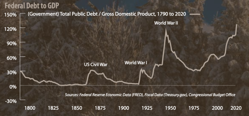
US public debt as a percentage of gross domestic product (GDP), is at an all-time high of 135.6%.12 US debt and leverage metrics were already relatively high at over 100% of GDP during a period of economic expansion prior to the onset of the coronavirus. Typically, a country’s debt and leverage metrics rise during periods of economic recessions or war; before this all-time high, US public debt after World War II reached its apex at 121% of GDP. We are now in uncharted territory. Government spending is projected to rise to address the pronounced economic impact of the pandemic and the tens of millions of unemployment claims over the last year.13
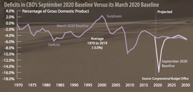
The Congressional Budget Office (CBO) assessed US deficit trends in their September 2020 publication. The CBO revised their April 2020 deficit projection of 4% to as much as 16%, the largest deficit since reaching nearly 30% during World War II.14 We believe that these projections dramatically understate US fiscal and debt-to-GDP metrics. It is reasonable to expect US fiscal policy to be accommodative to offset the deep economic impacts caused by the pandemic.
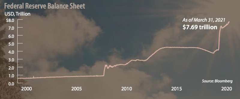
On December 16, 2020, the Federal Reserve reaffirmed its accommodative position by announcing plans to buy $120 billion in assets a month ($80 billion in US Treasurys and $40 billion in mortgages) while seeking to achieve maximum employment and an inflation rate of 2% in the long run. The Federal Open Market Committee commented “these asset purchases help foster smooth market functioning and accommodative financial conditions, thereby supporting the flow of credit to households and businesses.”15 The Fed vigorously embarked upon a massive asset purchase program in February 2020 that brought the federal deficit to a record $3.1 trillion during the 2020 fiscal year. The Fed’s actions led to a 42% increase in its balance sheet that as of March 31, 2021 stood in excess of $7.6 trillion.
The Fed modified its inflation policy framework in August of 2020. It will now target a 2% inflation average, rather than 2% as a fixed goal, allowing greater policy flexibility.16 Tyler Powell and David Wessel, writing for the Brookings Institution, theorize that the adoption of the new inflation policy suggests that the Fed will now hold off on tightening monetary policy, even if the unemployment rate falls back to where it was before the pandemic and inflation is projected to rise above 2%.17
Historically accommodative monetary and now loose fiscal policies are sowing the seeds of a US dollar decline – an excess supply of US dollars.
Exploring Your Options to Protect Your Purchasing Power
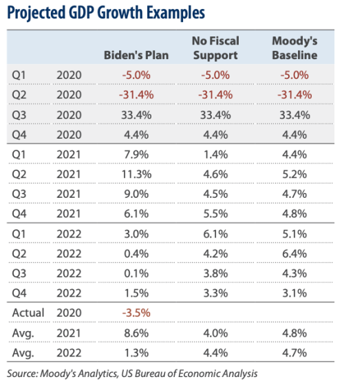
Moody’s Analytics estimates President Biden’s $1.9 trillion fiscal plan may generate average GDP growth of 8.6% for 2021 versus 4.0% with no fiscal stimulus at all. Moody’s Baseline anticipates GDP growth of 4.8% in 2021 based on a fiscal stimulus program of $750 billion.18 Again, these are all projections. Actual outcomes will vary since such programs face challenges associated with execution and rollout after legislation is passed. Also, President Biden’s plan doesn’t take into consideration a separate $2 trillion infrastructure plan that is in the queue.19
While the full extent of the various fiscal policies that could be cast during the Biden Presidency is unknown, repairing the economy along with increasing employment are top priorities. A bearish outlook for the US dollar has merit.
- Fiscal: Outlook for a loose fiscal policy is extremely likely. Current uncertainties remain on the size and the extent of what additional, if any, fiscal programs take place in the future.
- Monetary: Federal Reserve policymakers have confirmed an ongoing accommodative monetary policy. The Federal Reserve has engaged an accommodative policy ever since the GFC.
- Debt Trajectory: Currently, the US debt, as a percentage of GDP, exceeds levels observed during World War II. Both the debt and the deficit are expected to rise, and by a lot, dependent upon fiscal policy outcomes.
- Trade Deficit: There doesn’t appear to be clear guidance on the direction of the US trade deficit at this point, but that trade deficit does not seem to be a factor in the same way that it was from 2001 through 2008. Conditions may change if a large infrastructure bill is passed, requiring the acquisition of commodities and other goods needed to satisfy the projects.
A US dollar bear market can have meaningful adverse implications for investors and consumers. The good news is that we have a defensive toolkit.
Investors may want to consider owning non-US denominated securities to preserve their purchasing power. Such venues exist through diversified global bond funds that incorporate unhedged multi-currency exposures. These funds can help provide capital preservation to protect investors’ purchasing power against the rising prices of commodity items, such as gasoline, or the decline of the US dollar relative to other currencies. Alternatively, investors who prioritize capital appreciation rather than preservation may find diversified global equity funds that incorporate unhedged multi-currency exposures to be a favorable option.
What Can We Learn from the Past?
A US dollar bear market will undoubtedly have adverse implications for investors and consumers, particularly as it relates to changes in purchasing power. We can use history as our guide and look back to 2001–2008 to learn how asset classes performed during that period. Our aim is to help establish a playbook for investors to use, should the US dollar decline again. The adage “History may not repeat, but it does rhyme,” urges us to identify differences and similarities between the past and present.
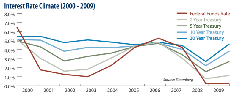
The federal funds rate plummeted between year-end 2000 and year-end 2001. Following this, US Treasury interest rates experienced an upward trajectory until the onset of the GFC, as shown in Interest Rate Climate (2000–2009). Since then, central banks from around the world have been engaged in various accommodative monetary programs to foster economic growth. Today’s interest rates are much lower than during 2001-2008 period.
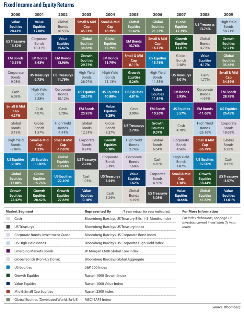
We compared risk-return attributes for the overlapping periods of 2001–2007 and 2001–2008 in order to contrast the risk-return attributes of these asset classes with and without the adverse impacts of the GFC.
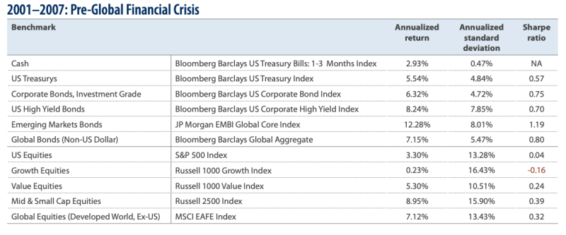
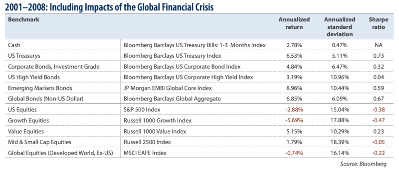
Sharpe ratio:
Developed by Nobel laureate William F. Sharpe, it helps investors evaluate a portfolio's return in terms of risk exposure. A higher Sharpe ratio indicates lower risk exposure relative to the return generated, while a lower ratio indicates relatively high risk exposure. The Sharpe ratio is calculated by subtracting the risk-free interest rate (e.g., that of US Treasury bills) from a portfolio's return, then dividing by the standard deviation of the portfolio's returns.
Standard Deviation:
The measure of how closely a set of data matches the mean (average) value of that data. The higher the standard deviation, the more spread out (or variable) the data points are. The lower the standard deviation, the more closely each data point matches the mean value of the group. Standard deviation can be used to measure the historical variability of a mutual fund's annual return.